Understanding PID Control in SWMM5 for a Weir

Understanding PID Control in SWMM5 for a Weir

• PID stands for Proportional-Integral-Derivative. It's a widely used control loop feedback mechanism that continuously calculates an "error" value as the difference between a desired setpoint and a measured process variable.¹ The controller then applies a correction based on proportional, integral, and derivative terms.
• Proportional (P): The output is proportional to the current error. A larger error produces a larger correction. kp is the gain.
• Integral (I): The output is proportional to the accumulated error over time. This helps to eliminate steady-state errors (the difference between the setpoint and the actual value that might persist with P control alone). ki is the gain and is often expressed as an integral time (in minutes or seconds), representing the time it would take for the integral term to equal the proportional term for a constant error.
• Derivative (D): The output is proportional to the rate of change of the error. This anticipates future error and dampens oscillations. kd is the gain and is often expressed as a derivative time (in minutes or seconds), representing the time it would take for the derivative term to equal the proportional term for a linearly changing error.

The SWMM 5 PID Rule

The provided rule effectively implements PID control to adjust the crest height of WEIR WEIR1@82309c-15009c to maintain a depth of 3 feet at NODE 82309c. Let's break it down:

RULE PID_Weir
; the PID controller adjusts the weir height to have a
;      depth of 3 feet in Node 82309e
IF NODE 82309c DEPTH 3
THEN WEIR WEIR1@82309c-15009c SETTING = PID 10 -.01 -.01
;                                         kp ki   kd
PRIORITY 1

• RULE PID_Weir: Defines the name of the rule.
• IF NODE 82309c DEPTH 3: This is the condition that triggers the rule. The error is the difference between the current depth and the target depth of 3 feet.
• THEN WEIR WEIR1@82309c-15009c SETTING = PID 10 -.01 -.01: This is the action. It sets the weir's SETTING (which likely represents the crest height relative to a datum or the degree of opening) based on the output of the PID function.
  • PID: This keyword indicates that a PID controller is being used.
  • 10 -.01 -.01: These are the PID parameters:
    • kp = 10: Proportional gain. A relatively high value, suggesting a strong response to the error.
    • ki = -0.01: Integral time (in minutes). A negative value is unusual in PID controllers and might lead to unexpected behavior or instability in this example. An integral time should almost always be positive. A very small value indicates a very strong integral action.
    • kd = -0.01: Derivative time (in minutes). A negative value is also unusual and could cause problems. A very small value represents a weak derivative action.
• PRIORITY 1: Assigns a priority to the rule. Lower numbers indicate higher priority.

Analysis and Recommendations

1. Negative ki and kd: The negative values for ki and kd are highly suspect. In most PID implementations, these values should be positive. Negative values could lead to instability and oscillations, as you observed. It is important to use positive ki and kd values or you get an unstable oscillation around the target depth.

2. Tuning the PID Parameters: Finding the optimal PID parameters often requires experimentation and tuning. The goal is to achieve a quick response to changes in water level while minimizing overshoot (going beyond the target depth) and oscillations.

   • High kp: The kp of 10 might be too high, potentially causing overreactions and oscillations.
   • Low or Negative ki: Try increasing the integral time (make it less negative or positive) to reduce oscillations and help the system settle at the target depth. Start with a small positive value, like 0.1 or 1, and adjust. For example, ki of 10 means an integral time of 10 minutes.
   • Low or Negative kd: Increase the derivative time (make it less negative or positive) to dampen oscillations. Start with a small positive value, like 0.01 or 0.1, and adjust. For example, a kd of 5 means a derivative time of 5 minutes.

3. Weir Setting Interpretation: The model assumes that the weir SETTING directly corresponds to the crest height adjustment. You should verify how the SETTING parameter is defined for your specific weir type in SWMM 5. The default setting is a fraction of fully open from 0 to 1.

Improved PID Rule (Example)

Here's an example of a revised rule with more typical PID parameter values:

RULE PID_Weir
IF NODE 82309c DEPTH 3
THEN WEIR WEIR1@82309c-15009c SETTING = PID 2 10 1
;                                         kp ki kd
PRIORITY 1

• kp = 2: Reduced proportional gain to lessen the initial response.
• ki = 10: Integral time set to 10 minutes (a positive value).
• kd = 1: Derivative time set to 1 minute (a positive value).

Tuning Process:

1. Start with the revised rule.
2. Run the simulation and observe the water level at NODE 82309c.
3. Adjust the parameters iteratively:
   • If the response is too slow: Increase kp slightly.
   • If there's overshoot or oscillations: Increase kd to dampen the response.
   • If the system doesn't settle exactly at 3 feet: Adjust ki (increase it to make the integral action stronger).
4. Repeat steps 2 and 3 until you achieve satisfactory performance.

In conclusion, the provided example demonstrates the powerful capability of SWMM 5 to implement PID control for regulating hydraulic structures. However, careful attention must be paid to the PID parameters to ensure stability and achieve the desired control objectives. The unusual negative values for ki and kd in the original rule should be corrected, and the parameters should be tuned iteratively to optimize the system's performance. You also need to make sure the Weir Setting in the THEN statement has the correct units of either fraction open or crest height.

 

 

How to Decide on a Time Step in InfoSWMM, ICM SWMM, or SWMM5

 How to Decide on a Time Step in InfoSWMM, ICM SWMM, or SWMM5

Understanding the Problem:

• Time Step Importance: The time step (also called the routing time step or computational time step) is a crucial parameter in dynamic hydraulic simulations. It determines how often the model calculates flow and depth in each element (links and nodes) of the network.
• Continuity Error: This error reflects the degree to which mass is conserved in the model. Ideally, the amount of water entering and leaving the system, plus any changes in storage, should balance out perfectly. A large continuity error indicates a problem with the simulation.
• Unstable Links: Unstable links exhibit rapid, unrealistic oscillations in flow or depth, often caused by an inappropriate time step or other model setup issues.

The Iterative Approach to Time Step Selection:

Step 1: Initial Guess and Evaluation

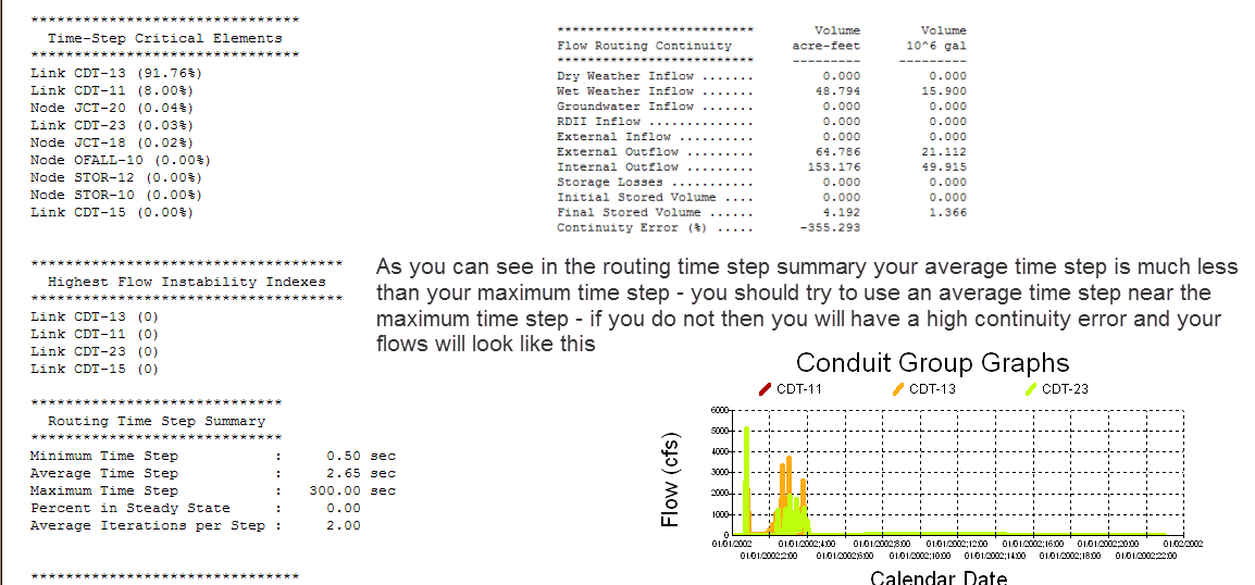
• Initial Guess (300 seconds): A 5-minute time step is a common starting point for some models, but as you found, it can be too large for systems with rapid changes in flow or complex hydraulics.
• Large Continuity Error and Instability: A large time step often leads to these problems because it cannot accurately capture the fast-paced changes in the system. The simulation essentially "skips over" important hydraulic events.
• Average Time Step as a Guide: The "average time step" reported by the simulation (2.6 seconds in your case) is a very useful indicator. It's the average time step that the model's internal variable time-step algorithm determined was needed to maintain numerical stability during the simulation. A large discrepancy between your chosen fixed time step and this average suggests that your fixed time step is too large.

Step 2: Refinement Based on Average Time Step

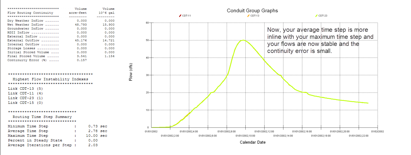
• New Time Step (10 seconds): You wisely chose a new time step that is closer to the reported average time step but still slightly larger. Using a time step very close to the minimum can significantly increase simulation time. It is better to be closer to the average time step.
• Reduced Continuity Error and Stable Flows: By using a smaller, more appropriate time step, you improved the accuracy of the simulation. The model can now better resolve the hydraulic changes, leading to a smaller continuity error and eliminating the unstable link flows.

Why this approach works:

• Variable Time Step Logic: SWMM and related software often use a variable time-step algorithm internally, even if you specify a fixed time step for reporting results. This algorithm adjusts the time step during the simulation based on the rate of change in flow and depth to maintain stability.
• Average Time Step as a Proxy: The average time step reported by the model reflects the time step that was generally needed to keep the simulation stable using this variable time-step logic. It provides valuable insight into the appropriate time step for your specific model.
• Iterative Improvement: Finding the optimal time step is often an iterative process. You start with an initial guess, evaluate the results, and then adjust the time step based on the model's behavior.

Additional Tips and Considerations:

• Courant Condition: The Courant condition is a theoretical stability criterion that relates the time step to the flow velocity and the length of the links. While SWMM's internal algorithms handle this to some extent, it is important to be aware of it. For explicit solvers, it is expressed as:
  • Δt ≤ Δx / c
  • where Δt is the time step, Δx is the link length, and c is the wave celerity (approximately the flow velocity in open channels).
  • If your links are very short and your velocities are very high a smaller time step will be needed.
• Model Complexity: More complex models (e.g., those with many interconnected ponds, rapid changes in flow, steep slopes, or complex control structures) generally require smaller time steps.
• Simulation Time: Smaller time steps increase simulation time. You need to find a balance between accuracy and computational efficiency.
• Output Interval: The reporting time step (output interval) can be larger than the routing time step. You might route with a 10-second time step but only save results every 5 or 15 minutes.
• Sensitivity Analysis: It's good practice to perform a sensitivity analysis by running your model with a few different time steps (e.g., 5, 10, and 15 seconds) to see how much the results change. If the results are not significantly affected, you can use the larger time step to save time.
• Other Model Issues: Keep in mind that continuity errors and instability can also be caused by other issues, such as incorrect boundary conditions, errors in the network connectivity, or unrealistic parameters.

In summary, the iterative approach you've described, guided by the average time step reported by the simulation, is a sound method for finding a suitable time step in InfoSWMM, ICM SWMM, or SWMM5. This approach helps to improve the accuracy and stability of your simulations while maintaining reasonable computational efficiency.